How a convolutional network classifies an image

Open the interactive demo →

This explanation is adapted from the article by CNN Explainer team, under the MIT license.

What is a Convolutional Neural Network? #

In machine learning, a classifier assigns a class label to a data point. For example, an image classifier produces a class label (e.g, bird, plane) for what objects exist within an image. A convolutional neural network, or CNN for short, is a type of classifier, which excels at solving this problem!

A CNN is a neural network: an algorithm used to recognize patterns in data. Neural Networks in general are composed of a collection of neurons that are organized in layers, each with their own learnable weights and biases. Let’s break down a CNN into its basic building blocks.

1. A tensor can be thought of as an n-dimensional matrix. In the CNN demo, tensors will be 3-dimensional with the exception of the output layer.
2. A neuron can be thought of as a function that takes in multiple inputs and yields a single output. The outputs of neurons are represented in the demo as the red → blue activation maps.
3. A layer is simply a collection of neurons with the same operation, including the same hyperparameters.
4. Kernel weights and biases, while unique to each neuron, are tuned during the training phase, and allow the classifier to adapt to the problem and dataset provided. They are encoded in the visualization with a yellow → green diverging colorscale. The specific values can be viewed in the Interactive Formula View by clicking a neuron or by hovering over the kernel/bias in the Convolutional Elastic Explanation View.
5. A CNN conveys a differentiable score function, which is represented as class scores in the visualization on the output layer.

If you have studied neural networks before, these terms may sound familiar to you. So what makes a CNN different? CNNs utilize a special type of layer, aptly named a convolutional layer, that makes them well-positioned to learn from image and image-like data. Regarding image data, CNNs can be used for many different computer vision tasks, such as image processing, classification, segmentation, and object detection.

In CNN Explainer, you can see how a simple CNN can be used for image classification. Because of the network’s simplicity, its performance isn’t perfect, but that’s okay! The network architecture, Tiny VGG, used in CNN Explainer contains many of the same layers and operations used in state-of-the-art CNNs today, but on a smaller scale. This way, it will be easier to understand getting started.

What does each layer of the network do? #

Let’s walk through each layer in the network. Feel free to interact with the interactive demo by clicking and hovering over various parts of it as you read.

Input Layer #

The input layer (leftmost layer) represents the input image into the CNN. Because we use RGB images as input, the input layer has three channels, corresponding to the red, green, and blue channels, respectively, which are shown in this layer. Use the color scale when you click on the Show detail control in the demo to display detailed information (on this layer, and others).

Convolutional Layers #

The convolutional layers are the foundation of CNN, as they contain the learned kernels (weights), which extract features that distinguish different images from one another—this is what we want for classification! As you interact with the convolutional layer, you will notice links between the previous layers and the convolutional layers. Each link represents a unique kernel, which is used for the convolution operation to produce the current convolutional neuron’s output or activation map.

The convolutional neuron performs an elementwise dot product with a unique kernel and the output of the previous layer’s corresponding neuron. This will yield as many intermediate results as there are unique kernels. The convolutional neuron is the result of all of the intermediate results summed together with the learned bias.

For example, let’s look at the first convolutional layer in the Tiny VGG architecture in the demo. Notice that there are 10 neurons in this layer, but only 3 neurons in the previous layer. In the Tiny VGG architecture, each output feature map combines contributions from all input channels, with a separate spatial kernel for each channel. Focusing on the output of the topmost convolutional neuron from the first convolutional layer, we see that there are 3 unique kernels when we hover over the activation map.

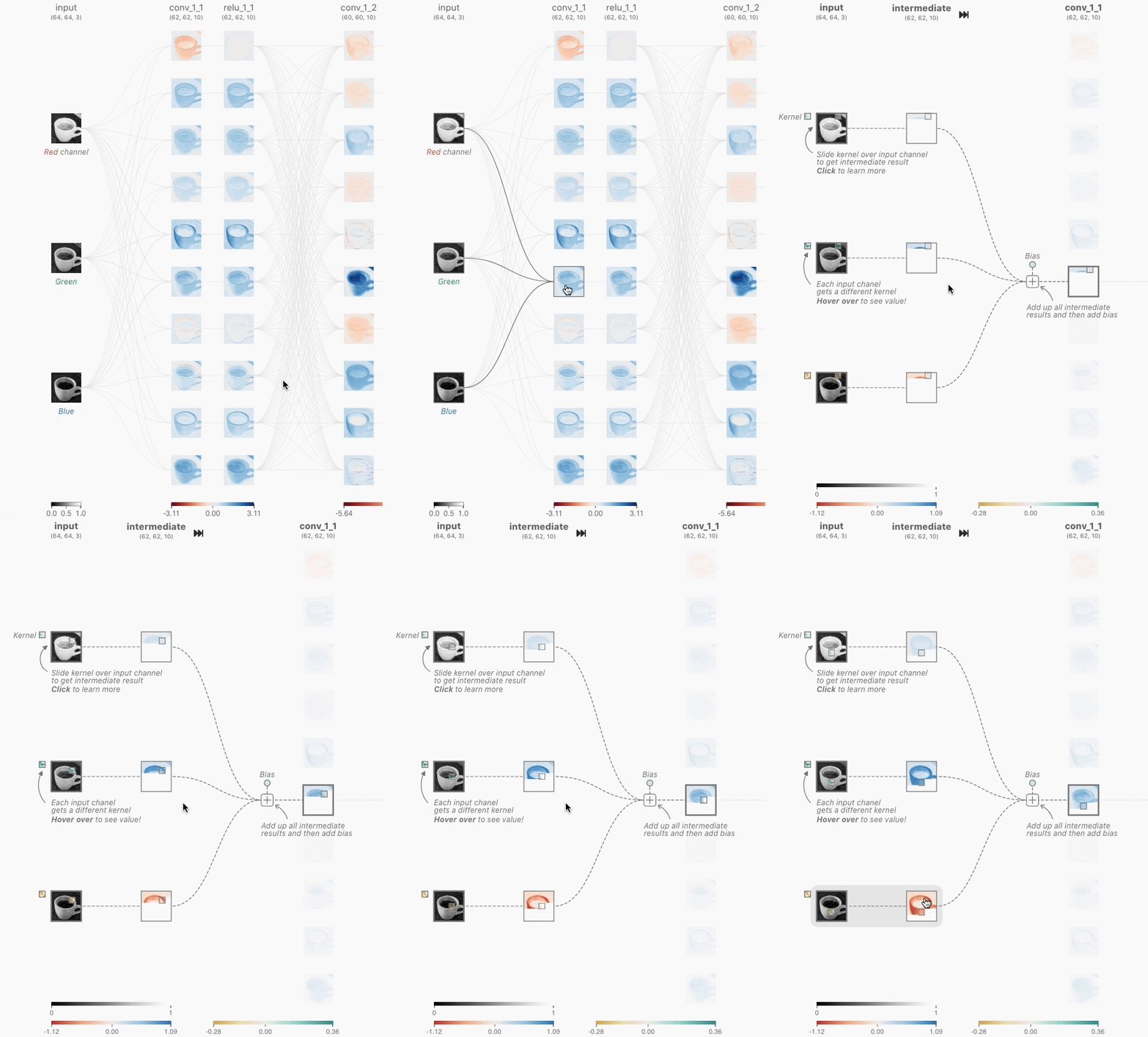
Figure 1. As you hover over the activation map of the topmost node from the first convolutional layer, you can see that 3 kernels were applied to yield this activation map. After clicking this activation map, you can see the convolution operation occuring with each unique kernel.

The size of these kernels is a hyper-parameter specified by the designers of the network architecture. In order to produce the output of the convolutional neuron (activation map), we must perform an elementwise dot product with the output of the previous layer and the unique kernel learned by the network. In TinyVGG, the dot product operation uses a stride of 1, which means that the kernel is shifted over 1 pixel per dot product, but this is a hyperparameter that the network architecture designer can adjust to better fit their dataset. We must do this for all 3 kernels, which will yield 3 intermediate results.

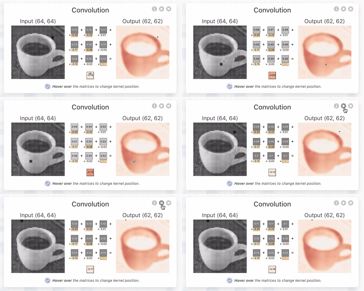
Figure 2. The kernel being applied to yield the topmost intermediate result for the discussed activation map.

Then, an elementwise sum is performed containing all 3 intermediate results along with the bias the network has learned. After this, the resulting 2-dimensional tensor will be the activation map viewable on the demo interface for the topmost neuron in the first convolutional layer. This same operation must be applied to produce each neuron’s activation map.

With some simple math, we are able to deduce that there are 3 x 10 = 30 unique kernels, each of size 3x3, applied in the first convolutional layer. The connectivity between the convolutional layer and the previous layer is a design decision when building a network architecture, which will affect the number of kernels per convolutional layer. Click around the visualization to better understand the operations behind the convolutional layer. See if you can follow the example above!

Understanding Hyperparameters #

Expand Kernel parameters in the demo to change the input size, padding, kernel size, and stride.

1. Padding is often necessary when the kernel extends beyond the activation map. Padding conserves data at the borders of activation maps, which leads to better performance, and it can help preserve the input's spatial size, which allows an architecture designer to build deeper, higher performing networks. There exist many padding techniques, but the most commonly used approach is zero-padding because of its performance, simplicity, and computational efficiency. The technique involves adding zeros symmetrically around the edges of an input. This approach is adopted by many high-performing CNNs such as AlexNet.
2. Kernel size, often also referred to as filter size, refers to the dimensions of the sliding window over the input. Choosing this hyperparameter has a massive impact on the image classification task. For example, small kernel sizes are able to extract a much larger amount of information containing highly local features from the input. As you can see on the interactive demo, a smaller kernel size also leads to a smaller reduction in layer dimensions, which allows for a deeper architecture. Conversely, a large kernel size extracts less information, which leads to a faster reduction in layer dimensions, often leading to worse performance. Large kernels are better suited to extract features that are larger. At the end of the day, choosing an appropriate kernel size will be dependent on your task and dataset, but generally, smaller kernel sizes lead to better performance for the image classification task because an architecture designer is able to stack more and more layers together to learn more and more complex features!
3. Stride indicates how many pixels the kernel should be shifted over at a time. For example, as described in the convolutional layer example above, Tiny VGG uses a stride of 1 for its convolutional layers, which means that the dot product is performed on a 3x3 window of the input to yield an output value, then is shifted to the right by one pixel for every subsequent operation. The impact stride has on a CNN is similar to kernel size. As stride is decreased, more features are learned because more data is extracted, which also leads to larger output layers. On the contrary, as stride is increased, this leads to more limited feature extraction and smaller output layer dimensions. One responsibility of the architecture designer is to ensure that the kernel slides across the input symmetrically when implementing a CNN. Use Kernel parameters in the demo to compare the output dimensions for different stride settings.

Activation Functions #

ReLU #

Neural networks are extremely prevalent in modern technology—because they are so accurate! The highest performing CNNs today consist of an absurd amount of layers, which are able to learn more and more features. Part of the reason these groundbreaking CNNs are able to achieve such tremendous accuracies is because of their non-linearity. ReLU applies much-needed non-linearity into the model. Non-linearity is necessary to produce non-linear decision boundaries, so that the output cannot be written as a linear combination of the inputs. If a non-linear activation function was not present, deep CNN architectures would devolve into a single, equivalent convolutional layer, which would not perform nearly as well. The ReLU activation function is specifically used as a non-linear activation function, as opposed to other non-linear functions such as Sigmoid because it has been empirically observed that CNNs using ReLU are faster to train than their counterparts.

The ReLU activation function is an elementwise mathematical operation:

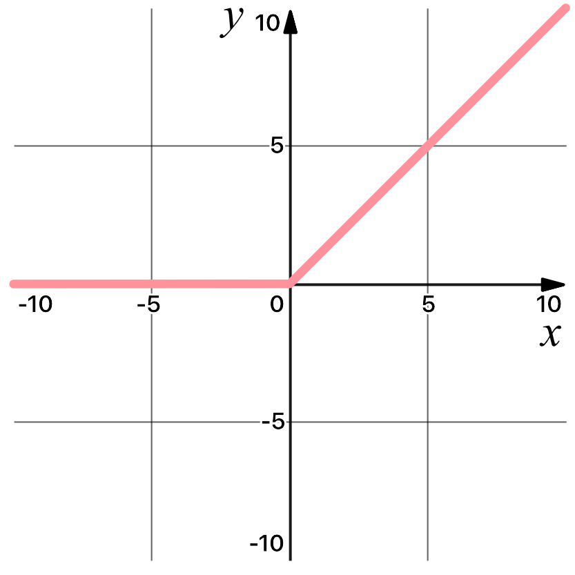
Figure 3. The ReLU activation function graphed, which disregards all negative data.

This activation function is applied elementwise on every value from the input tensor. For example, if applied ReLU on the value 2.24, the result would be 2.24, since 2.24 is larger than 0. You can observe how this activation function is applied by clicking a ReLU neuron in the network in the demo. The Rectified Linear Activation function (ReLU) is performed after every convolutional layer in the network architecture shown in the demo. Notice the impact this layer has on the activation map of various neurons throughout the network!

Softmax #

A softmax operation serves a key purpose: making sure the CNN outputs sum to 1. Because of this, softmax operations are useful to scale model outputs into probabilities. Clicking on the last layer reveals the softmax operation in the network. Notice how the logits after flatten aren’t scaled between zero to one. For a visual indication of the impact of each logit (unscaled scalar value), they are encoded using a light orange → dark orange color scale. After passing through the softmax function, each class now corresponds to an appropriate probability!

You might be thinking what the difference between standard normalization and softmax is—after all, both rescale the logits between 0 and 1. Remember that backpropagation is a key aspect of training neural networks—we want the correct answer to have the largest “signal.” By using softmax, we are effectively “approximating” argmax while gaining differentiability. Rescaling doesn’t weigh the max significantly higher than other logits, whereas softmax does. Simply put, softmax is a “softer” argmax—see what we did there?

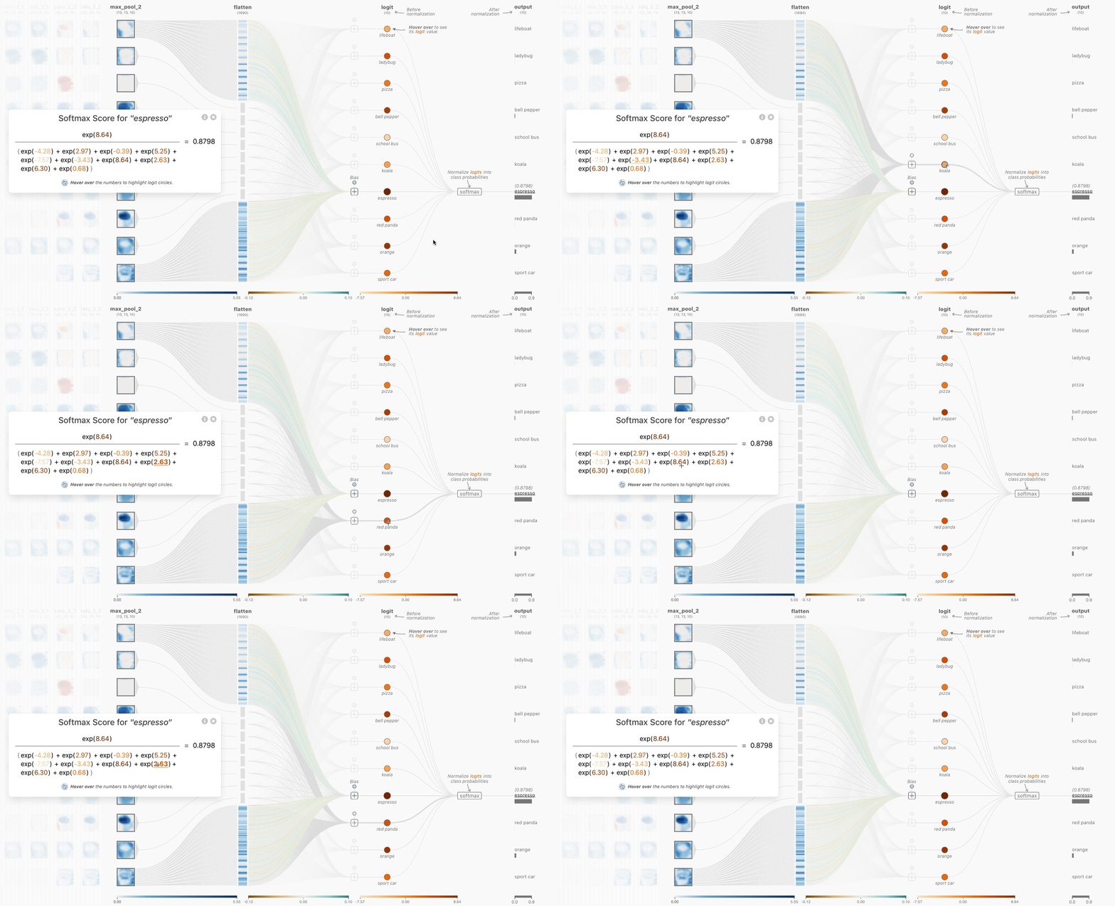
Figure 4. The Softmax Interactive Formula View allows a user to interact with both the color encoded logits and formula to understand how the prediction scores after the flatten layer are normalized to yield classification scores.

Pooling Layers #

There are many types of pooling layers in different CNN architectures, but they all have the purpose of gradually decreasing the spatial extent of the network, which reduces the parameters and overall computation of the network. The type of pooling used in the Tiny VGG architecture in the demo is Max-Pooling.

The Max-Pooling operation requires selecting a kernel size and a stride length during architecture design. Once selected, the operation slides the kernel with the specified stride over the input while only selecting the largest value at each kernel slice from the input to yield a value for the output. This process can be viewed by clicking a pooling neuron in the network in the demo.

In the Tiny VGG architecture in the demo, the pooling layers use a 2x2 kernel and a stride of 2. This operation with these specifications results in the discarding of 75% of activations. By discarding so many values, Tiny VGG is more computationally efficient and avoids overfitting.

Flatten Layer #

This layer converts a three-dimensional layer in the network into a one-dimensional vector to fit the input of a fully-connected layer for classification. For example, a 5x5x2 tensor would be converted into a vector of size 50. The previous convolutional layers of the network extracted the features from the input image, but now it is time to classify the features. We use the softmax function to classify these features, which requires a 1-dimensional input. This is why the flatten layer is necessary. This layer can be viewed by clicking any output class.

Using the demo #

Choose an image or upload one with the plus button. Click a feature map to inspect the operation that produced it, then use the layer controls to play or pause the calculation.

Show detail displays layer dimensions and color scales. The scale selector switches between unit, module, and global comparisons. Expand Kernel parameters to change padding, stride, and kernel size on the smaller matrix example.

How is CNN Explainer implemented? #

CNN Explainer uses TensorFlow.js, an in-browser GPU-accelerated deep learning library to load the pretrained model for visualization. The entire interactive system is written in Javascript using Svelte as a framework and D3.js for visualizations. You only need a web browser to get started learning CNNs today!

Who developed CNN Explainer? #

CNN Explainer was created by Jay Wang, Robert Turko, Omar Shaikh, Haekyu Park, Nilaksh Das, Fred Hohman, Minsuk Kahng, and Polo Chau, which was the result of a research collaboration between Georgia Tech and Oregon State. We thank Anmol Chhabria, Kaan Sancak, Kantwon Rogers, and the Georgia Tech Visualization Lab for their support and constructive feedback. This work was supported in part by NSF grants IIS-1563816, CNS-1704701, NASA NSTRF, DARPA GARD, gifts from Intel, NVIDIA, Google, Amazon.