The useful starting point in OpenAI’s September 2026 Navier–Stokes paper is a small region of fluid that contracts while its characteristic velocity increases. Its radius shrinks faster than its height. That makes the core increasingly slender, even though both dimensions approach zero.
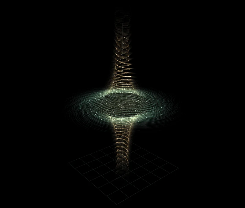
The WebGL study makes those competing scales visible. It adapts the CC0 vortex illustration by 3d retro graphics, using the leading geometry from section 2.1 of the paper.
Read the theorem before the animation #
The paper considers three-dimensional incompressible flow with positive viscosity and an external force:
Theorem 1.1 starts the fluid from rest. For every positive viscosity, the authors construct a smooth force, compactly supported in space and time, and a solution whose maximum velocity becomes unbounded as time approaches 1. Its kinetic energy remains uniformly bounded before that time. The paper establishes the breakdown alternatives (C) and (D) in Clay’s problem statement, for the whole space and the periodic torus respectively.
The forcing hypothesis matters. This Navier–Stokes construction uses a force; the companion Euler result concerns an unforced, inviscid flow. They are separate theorems. OpenAI publishes Lean formalizations of both in its research repository.
Clay’s September 11 announcement describes the problem as apparently settled and says the formal evaluation will proceed deliberately. That is the status of the result at the time of this note.
Two lengths, one shrinking core #
Write the remaining time as . Section 2.1 gives the leading radial and axial scales:
Here means the quantities agree up to positive factors independent of . Both exponents are positive, so both lengths shrink. Their ratio tells a different story:
The aspect ratio grows. This is easy to misread when the camera follows the core: a uniform zoom that holds the radial scale steady makes the axis appear to lengthen. Turn off Follow core to watch the whole structure contract in a fixed frame.
The demo uses the illustrative value and an approach coordinate . Each unit of the slider reduces the remaining time by a factor of ten. At , the radial scale is of its initial value, but the axial-to-radial scale ratio has increased by only about 15%. The different rates matter asymptotically; the paper’s small exponent makes their visible separation gradual.
Large speed can coexist with small energy #
The characteristic azimuthal and axial speeds scale as . The core volume scales as . Multiplying volume by squared speed gives the leading core-energy scale:
That exponent is positive in the stated range of . The energy in the core therefore tends to zero even as its largest speeds diverge. An integral bound can hide increasingly intense behavior concentrated in a sufficiently small region. For anyone used to system-wide averages, the distinction between an aggregate and a local maximum is familiar; here it is part of the mathematical construction.
The shrinking core is a region defined by the flow’s changing scales. It is not a sealed parcel of fluid. Incompressibility preserves the volume of material parcels, while fluid moves into and out of this region.
The difficult part is the residual #
A contracting vortex is only the beginning. Given velocity and pressure, one can define the force to be whatever remains in the momentum equation. The hard requirement is that this residual force stays smooth through the singular time.
The paper first constructs an axisymmetric background. Connecting its inner core to an exterior flow leaves a singular momentum imbalance in the surrounding annulus. Spatially oscillatory pulses supply additional momentum flux through the nonlinear term. Their averaged quadratic products cancel the leading imbalance; further corrections control the remaining singular errors. The resulting force extends smoothly even though the velocity blows up.
Those pulses and corrections are where the geometric picture becomes a proof. The demo draws parametric helices with the paper’s leading contraction scales. Its particles are illustrative tracers, and its colors encode normalized radius. It does not integrate the Navier–Stokes equations or compute the correction fields.
A useful way to explore #
Pause the animation and move the approach slider. Compare Follow core with a fixed frame at the same slider position. Read the grid spacing as you zoom: equal distances on the screen represent progressively smaller physical lengths. Drag the scene, or focus the canvas and use the arrow keys, to inspect the axis.
The finite slider range stops before the singular time. It is enough to inspect the geometry; the statement about the limit comes from the estimates in the paper.
Sources #
- OpenAI, Finite time blowup for Navier–Stokes, especially Theorem 1.1 and sections 2–3.
- OpenAI, Navier–Stokes and Euler formalizations.
- Clay Mathematics Institute, Navier–Stokes announcement, September 11, 2026.
- 3d retro graphics, Vortex illustration, CC0 1.0.